Calculating trigger efficiencies
This section introduces the relevant background required to understand trigger efficiency calculations. First, the Run 3 LHCb trigger and dataflow are briefly introduced. Then the data-driven TISTOS method is introduced and propagation of uncertainties on trigger efficiencies is discussed. Finally, the mitigation of backgrounds by means of sideband subtraction, fit-and-count and sPlot approaches is presented.
Data-driven efficiencies with the TISTOS method
TISTOS is a data-driven method for determining trigger efficiencies, discussed (including full proof) in full in Ref. 1. This method is briefly outlined below.
Ideally, the efficiency of a trigger selection could be calculated as
where \(N_\mathrm{Total}\) is the total number of events within the acceptance (i.e., which could be triggered) and \(N_\mathrm{Trig}\) is the number of events which are triggered on. More frequently \(\varepsilon_\mathrm{Trig}\) is defined in terms of the number of events in a sample subject to some form of selection, \(N_\mathrm{Sel}\). The Trig, TIS, TOS and TISTOS categories discussed here are all assumed to be conditional on this selection, with the \(\mathrm{\vert Sel}\) generally dropped for convenience.
However, since triggering is a destructive process, \(N_\mathrm{Total}/N_\mathrm{Sel}\) are not known quantities in data (in simulation we can keep this information, which makes our lives much easier). As such, we will need to get a bit more creative.
Defining the TIS and TOS categories
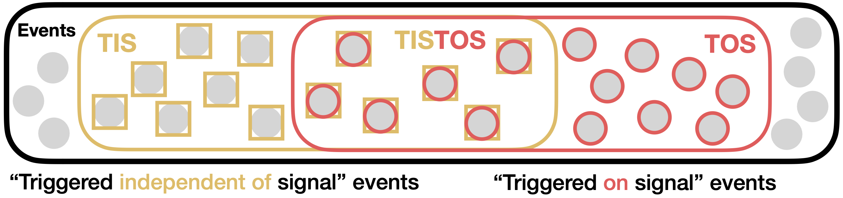
We start by defining categories in terms of the trigger response on each event and with respect to a given signal (i.e., a particle in the channel of interest):
- Trig.: The trigger fires on the event.
- TOS: The presence of the signal causes the trigger to fire on the event. Specifically, at least 70% of hits in the reconstructed trigger candidates are hits associated with the signal.
- TIS: The trigger fires on the event regardless of the signal. Specifically, if any of the reconstructed trigger candidates share fewer than 1% of hits with the signal.
- TISTOS: The event is both TIS and TOS.
From categories to efficiencies
Each of the TIS/TOS/TISTOS categories then has a corresponding efficiency:
These are particularly useful because \(\varepsilon_\mathrm{Trig.}\) can be expanded as
Whilst \(\varepsilon_\mathrm{TIS}\) was previously defined in terms of \(N_\mathrm{Sel}\), this efficieny can be defined within the TOS subsample as
which is equivalent to \(\varepsilon_\mathrm{TIS}\) under the assumption that \(\varepsilon_\mathrm{TIS}\) of any subsample is identical to that of the full sample. Plugging this into the expression for \(\varepsilon_\mathrm{Trig.}\) yields the final expression for \(\varepsilon_\mathrm{Trig.}\) (as implemented in the tools),
A frequently-used proxy for this trigger efficiency, \(\varepsilon_\mathrm{TOS}\) can be defined in a similar way to \(\varepsilon_\mathrm{TIS}\):
equivalent to \(\varepsilon_\mathrm{TOS}\) under a similar assumption that \(\varepsilon_\mathrm{TOS}\) is the same in the whole sample as in any subsample. Both \(\varepsilon_\mathrm{TOS}\) and \(\varepsilon_\mathrm{TIS}\) are also implemented in the tool.
Mitigating correlation between TIS and TOS
The assumptions of TIS/TOS subsample-independence are not strictly true as, the signal and the rest of the event are frequently correlated, e.g.,, in the case of \(B\) mesons, where the \(b\bar{b}\) are produced as a pair and hence both \(B\) are correlated. This correlation can be circumvented by calculating the counts detailed above in sufficiently small phase space bins. Performing such a binning, the expression for \(\varepsilon_\mathrm{Trig.}\) becomes
Note
For more details and a derivation of the error propagation for \(\varepsilon_\mathrm{Trig.}\) (also as implemented in the tools), it is highly recommended that you read Ref. 1
Propagation of statistical uncertainties
To appropriately handle the statistical uncertainty on an efficiency, the LHCb Statistics Guidelines recommend applying the Wilson interval method to compute lower and upper limits at the 68% confidence level. This approach provides appropriate coverage across the full range of 0 to 1; however, this assumes that the uncertainties on the numerator and denominator are their respective square roots. This assumption can be invalid for a number of reasons, for example for yields extracted from likelihood fits (as per the fit-and-count method discussed below), or for the denominator of \(\varepsilon_\mathrm{Trig.}\) which is formed of several overlapping terms (the treatment of which is discussed in detail in Ref. 1).
To account for non-Poissonian contributions to the efficiency numerator and denominator, a generalised Wilson interval is used instead of the standard Wilson interval implemented in ROOT.TEfficiency.
The generalised Wilson interval is introduced by H. Dembinski and M. Schmelling in Ref. 2 (specifically Eq. 44).
This has been implemented in TriggerCalib in the wilson function of triggercalib.utils.stats
A standard Wilson interval or the direct propagation of Poissonian errors (per 1) can be enabled by the uncertainty_method argument in HltEff.
Mitigation of backgrounds
Most samples from which we would wish to extract a trigger efficiency are not entirely signal and instead contain some background component(s). To compute signal efficiencies in such samples, the background(s) must be mitigated. Three methods for mitigating background are presented here: sideband subtraction, fit-and-count and sPlot. The validity and limitations of each method are also discussed below.
This section will make frequent use of the terms control variable(s) and discriminating variable(s). The control variable is the variable we are interested in making some measurement in, e.g., the transverse momentum of a \(B^0\), whilst the discriminating variable is the variable which is used to make a distinction between signal and background, e.g., invariant mass of \(B^0\) products.
Subtraction of sideband density
For well-behaved (near-linear) backgrounds lying beneath the signal in the discriminating variable distribution, the background beneath the signal can be estimated from the sidebands: regions in the discriminating variable well-separated from the signal region. The background density is calculated by counting the number of events in the sidebands and normalising by the width of the sidebands. This density is converted to a background count by multiplying by the width of the region of interest (either the whole signal region or a single bin). The signal count in the region of interest can then be calculated by simply subtracting this estimated background count. This can be repeated per-bin in the control variable(s) to subtract the background density in every bin.
Per-bin fitting and counting (fit-and-count)
More complicated backgrounds, e.g., peaking backgrounds overlapping with the signal, cannot be well-mitigated using sideband subtraction. Instead, a more thorough approach is involved, wherein an extended fit is performed to the discriminating variable, with a signal component and one or more background components. The yield of the signal component can then be taken to be the signal count. This too can be repeated per-bin in the control variable(s) to build up a useful histogram of signal counts. This is more precise but typically also more computationally expensive than sideband subtraction and requires bins to be coarse enough that all fits converge.
Weighting from global fits with sPlot
A compromise with the fit-and-count approach can be found in the sPlot method, in which per-event weights are computed from a fit to the discriminating variable which is global in the control variable(s). These weights can then be counted when binning the control variable(s) to obtain a signal histogram. This approach is only valid if all components of the fit are uncorrelated between discriminating and control variables.
References
-
S. Tolk et al., Data driven trigger efficiency determination at LHCb (LHCb-PUB-2014-039), 2014 ↩↩↩↩
-
H. Dembinski and M. Schmelling, Bias, variance, and confidence intervals for efficiency estimators in particle physics experiments arXiv:2110.00294, 2022 ↩